Getting started

This guide walks through opening your first DAS file in DASexplorer and navigating the main interface.

Launch the application

Once you have DASexplorer installed, activate the appropriate environment and launch the interface with:

dasexplorer

Open a file

1. Select the profile matching your interrogator and data format (see Reading profiles)
2. Select a stride value (default stride=1). This applies a channel stride (spatial decimation) to reduce memory load
3. Go to File > Open file... or press the Select file... button

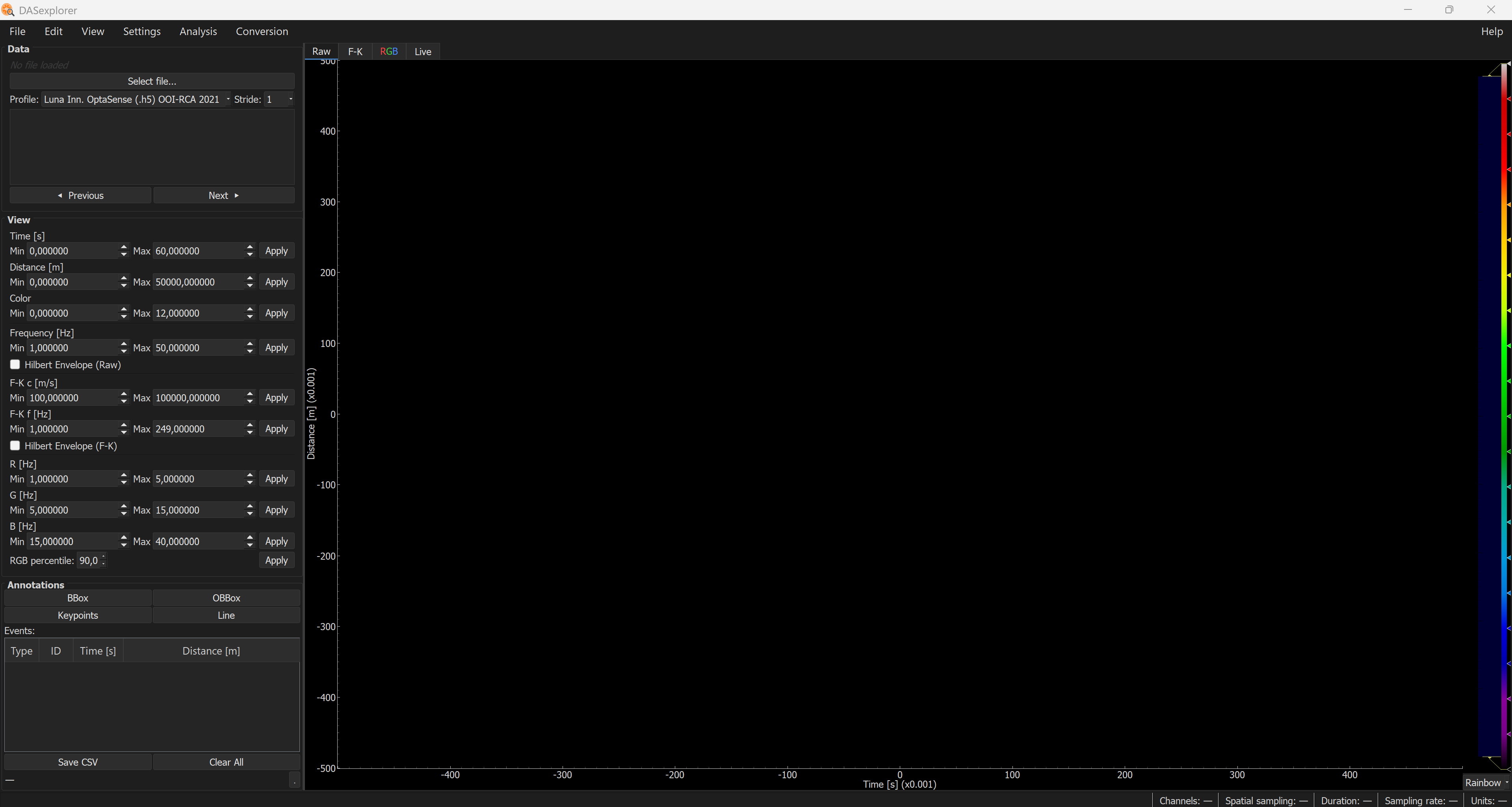
The top-right panel shows the loaded file highlighted in blue. Just below it, you'll see the list of files in that same directory with the same extension. The Previous and Next buttons let you step backward or forward through the file list. Double-clicking a file in the list loads it.

Tip

Use read_dmin_m / read_dmax_m in the configuration profile to restrict the spatial range loaded into memory if you don't need to view the full distance range. Setting them to null loads the full cable — see Create reading profiles. Increasing the stride also helps manage memory issues.

Example datasets

To start experimenting with the interface, we recommend using public example datasets that already have default read profiles configured:

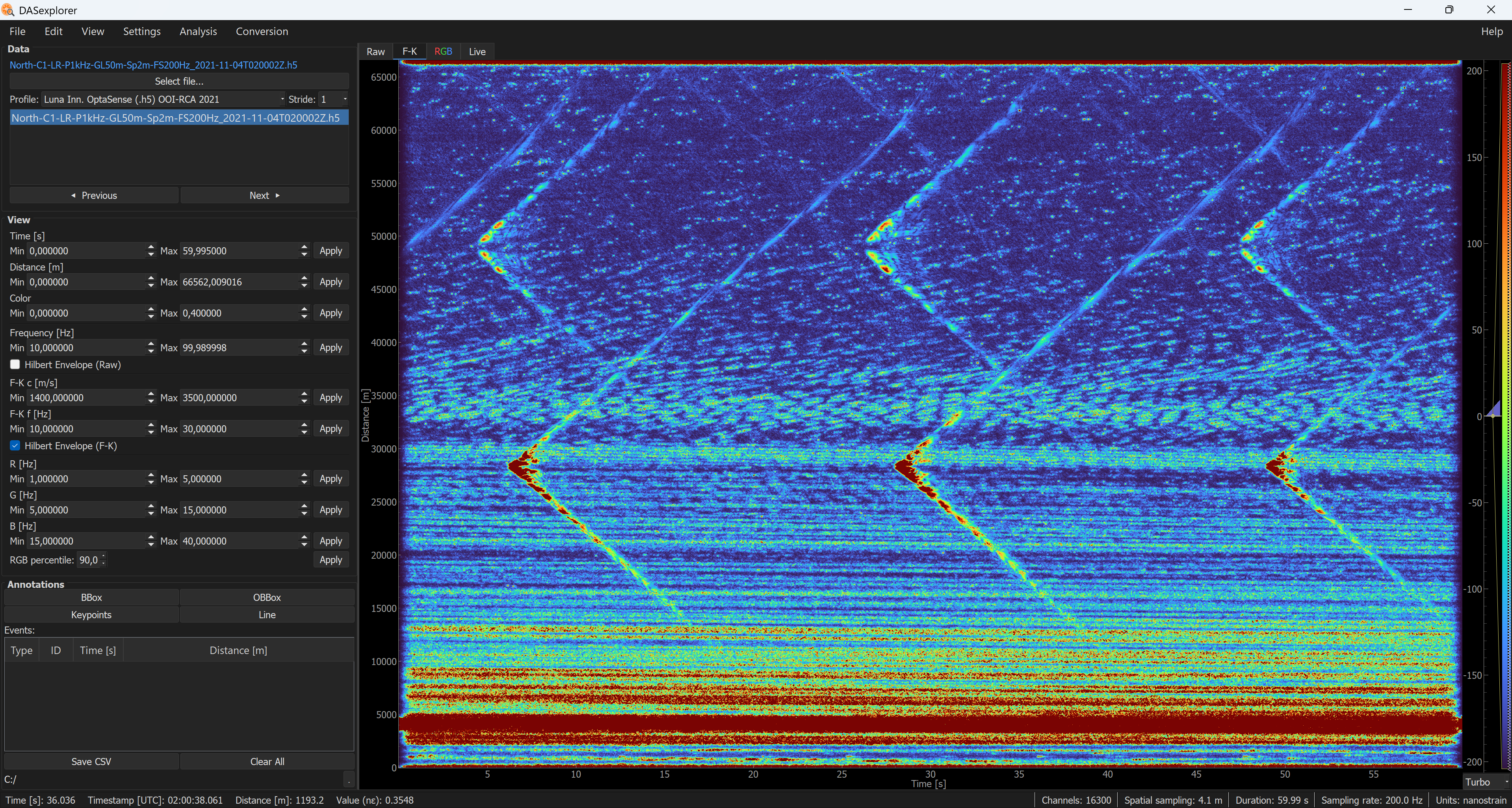
OptaSense — OOI Regional Cabled Array (F-K visualization)

Interrogator: Luna Innovations OptaSense Format: HDF5 (.h5) Dataset: Rapid: A Community Test of Distributed Acoustic Sensing on the Ocean Observatories Initiative Regional Cabled Array Example file: North-C1-LR-P1kHz-GL50m-Sp2m-FS200Hz_2021-11-04T020002Z.h5

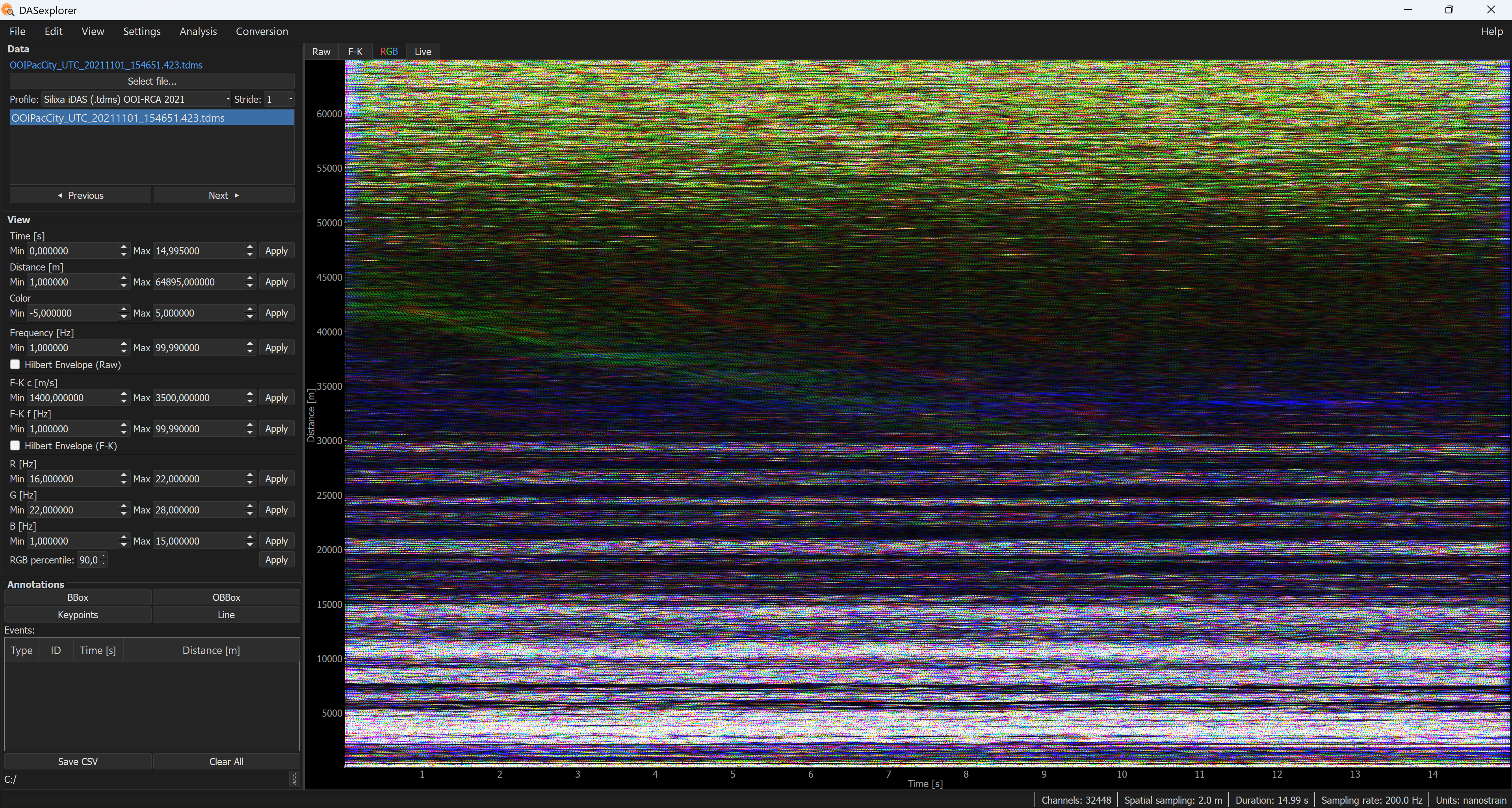
Silixa iDAS — OOI Regional Cabled Array (RGB visualization)

Interrogator: Silixa iDAS Format: TDMS (.tdms) Dataset: Rapid: A Community Test of Distributed Acoustic Sensing on the Ocean Observatories Initiative Regional Cabled Array Example file: OOIPacCity_UTC_20211101_163806.423.tdms

OptoDAS — Svalbard, Norway (raw visualization)

Interrogator: Alcatel Submarine Networks OptoDAS Format: MATLAB (.mat), processed Dataset: Longyearbyen, Svalbard (Norway) 2020 — DAS4Whales: Svalbard distributed acoustic sensing dataset for baleen whale monitoring Example file: 20200627_052441_ch10001_to_ch15000_whale_raw_L160s.mat

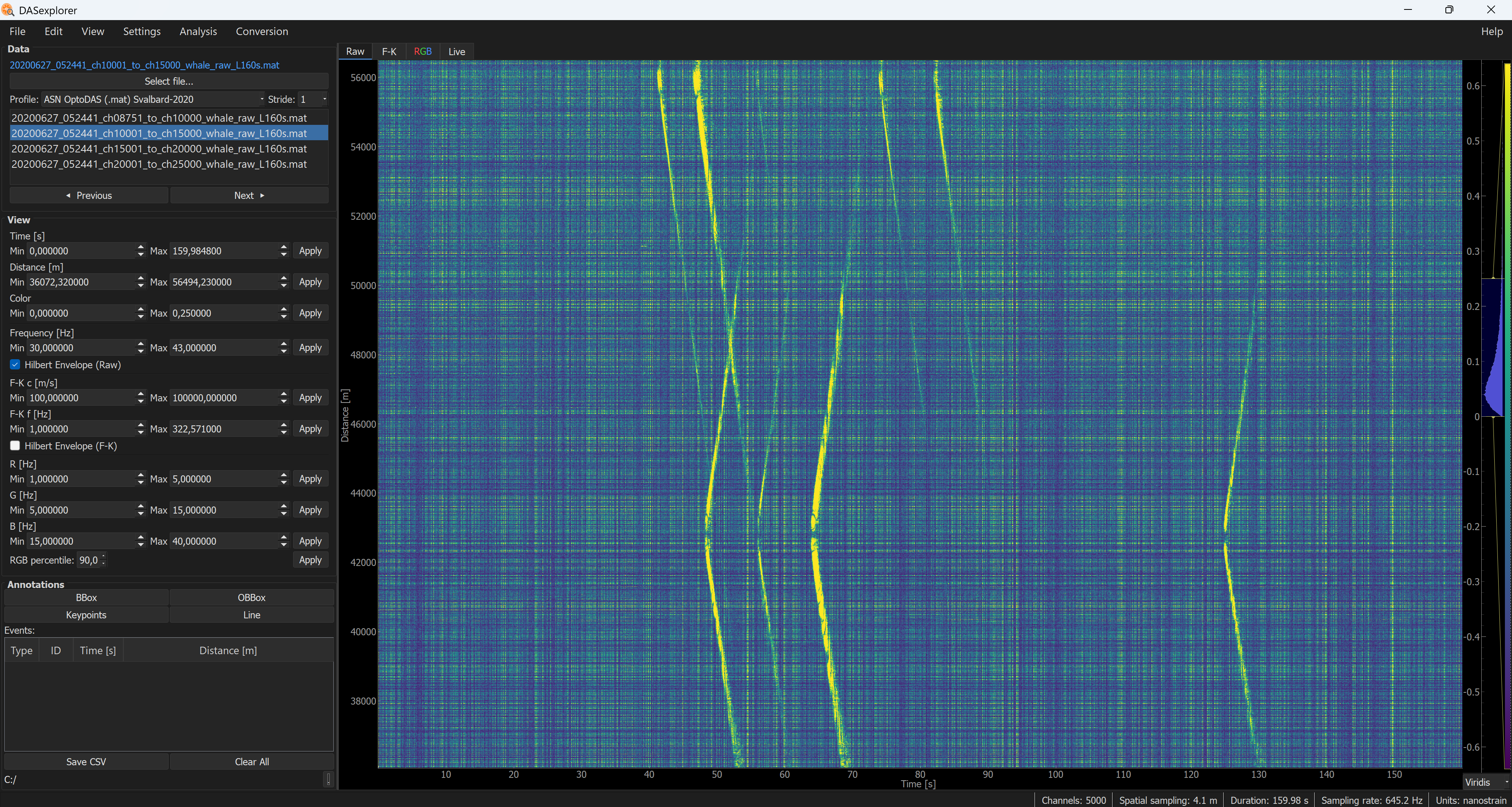
As you can see, each reading profile sets its own default visualisation values for the left panel — colour scale, bandpass filter range, F-K velocity bounds, RGB frequency bands, and so on. These are loaded automatically when a file is opened with that profile. You can adjust any of them interactively; to reset to the profile defaults, go to File → Refresh.

Warning

Keep in mind when working with large datasets: processed visualizations (i.e. F-K and RGB) are not precomputed by default, unless specified in the configuration profile. These visualizations are only calculated when you click the F-K or RGB tab, or press Apply on one of their parameters. It is therefore recommended to select the desired visualization values before rendering a processed view.

You can adjust visualization values in the left panel to customize, for example, minimum/maximum time, minimum/maximum distance, dynamic range, band-pass filter, and envelope on/off. If at any point you want to return to the configuration profile's default values, go to File > Refresh.

Channel stride

The Stride combo in the top-left panel controls spatial decimation: a stride of N loads every Nth channel, reducing memory use by a factor of N.

• Stride 1 — all channels (full resolution)
• Stride 2 — every other channel (half the channels)
• Stride 10 — one channel in ten (useful for very dense arrays such as Silixa iDAS at 2 m spacing)

The stride can also be changed after loading a file. If the new stride is a multiple of the current one, the subsampling is applied in memory instantly. Otherwise, the file is reloaded from disk with the new stride. The status bar at the bottom shows a message when the operation completes.

Tip

For large datasets (tens of thousands of channels), start with a high stride for a quick overview, then reload at stride 1 once you have identified the region of interest.

Additional information

The bottom-right panel shows the main metadata of the loaded file: Channels, Spatial sampling, Duration, Sampling rate, and Units.

Moving the mouse over the t-x waterfall (bottom left) displays the relative time, timestamp (UTC), distance, and waterfall value at the pointer's location.

Warning

When a process is running in the background, information about it is printed at the bottom left. It's recommended to wait until the process finishes to avoid blocking the interface.

The bottom-right panel also has a button showing the current colormap. You can choose between: Rainbow (recommended), Turbo, Grays, Viridis, Magma, and Seismic.

The widget on the right lets you equalize the histogram to adjust the color distribution in your visualization.

Color themes

You can choose between two themes, "dark" or "light", under View > Theme.

Export raw data

If you want to share an example dataset with a colleague who doesn't use DASexplorer, or want to plot your data in Python or MATLAB, a good way to do this is to export it as NPZ or MAT. To do so, go to:

File > Save as NPZ or File > Save as MAT

You can re-import these files with File > Import from NPZ or File > Import from MAT.